Using NetworkX to Plot Graphs

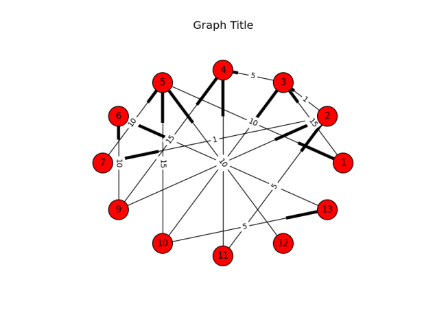
I’ve previously mentioned graphviz for plotting graphs. In truth, these resemble flowcharts. To create something that looks like a more traditional vertex and edge representation, you might consider NetworkX.

Whereas graphviz is a fairly general purpose utility that is not specific to Python and is developed around the well-defined DOT-format, NetworkX is Python specific but creates very nice graphics. It’s also significantly easier to get something that’s acceptable while probably minimizing the amount of time that you have to monkey with it. With that said, there are multiple layout algorithms that you can invoke to calculate the positions of the elements in the output image, and the only apparent way to get a consistent, well-organized/balanced representation seems to arrange them using the circular layout.

Digraph example:

import networkx as nx
import matplotlib.pyplot as plt

def _main():
    g = nx.DiGraph()

    g.add_edge(2, 3, weight=1)
    g.add_edge(3, 4, weight=5)
    g.add_edge(5, 1, weight=10)
    g.add_edge(1, 3, weight=15)

    g.add_edge(2, 7, weight=1)
    g.add_edge(13, 6, weight=5)
    g.add_edge(12, 5, weight=10)
    g.add_edge(11, 4, weight=15)

    g.add_edge(9, 2, weight=1)
    g.add_edge(10, 13, weight=5)
    g.add_edge(7, 5, weight=10)
    g.add_edge(9, 4, weight=15)

    g.add_edge(10, 3, weight=1)
    g.add_edge(11, 2, weight=5)
    g.add_edge(9, 6, weight=10)
    g.add_edge(10, 5, weight=15)

    pos = nx.circular_layout(g)

    edge_labels = { (u,v): d['weight'] for u,v,d in g.edges(data=True) }

    nx.draw_networkx_nodes(g,pos,node_size=700)
    nx.draw_networkx_edges(g,pos)
    nx.draw_networkx_labels(g,pos)
    nx.draw_networkx_edge_labels(g,pos,edge_labels=edge_labels)

    plt.title("Graph Title")
    plt.axis('off')

    plt.savefig('output.png')
    plt.show()

if __name__ == '__main__':
    _main()

Notice that NetworkX depends on matplotlib to do the actual drawing. The boots (highlighted parts on the edges) represent directedness.

Output:

NetworkX

As I said before, it’s easier to get a nicer representation, but it appears that this is at the cost of flexibility. Notice that in the image, there’s a a tendency to overlap. In fact, all of the edge-labels are dead-center. Since the nodes are arranged in a circle, all edges that cross from one side to another will have labels that overlap in the middle. Technically you can adjust whether the label is left, middle, or right, but it’s limited to that (rather than being calculated on the fly).

A Complete Huffman Encoder Implementation

I’ve written a Huffman implementation for the purpose of completely showing how to build the frequency-table, Huffman tree, encoding table, as well as how to serialize the tree, store the tree and data to a file, restore both structures from a file, decode the data using the tree, and how to make this more fun using Python.

This is the test code (test_steps):

clear_bytes = test_get_data()
_dump_hex("Original data:", clear_bytes)

tu = TreeUtility()

# Build encoding table and tree.

he = Encoding()
encoding = he.get_encoding(clear_bytes)

print("Weights:n{0}".format(pprint.pformat(encoding.weights)))
print('')

print("Tree:")
print('')

tu.print_tree(encoding.tree)
print('')

flat_encoding_table = { 
    (hex(c)[2:] + ' ' + chr(c).strip()): b
    for (c, b) 
    in encoding.table.items() }

print("Encoding:n{0}".format(pprint.pformat(flat_encoding_table)))
print('')

# Encode the data.

print("Encoded characters:nn{0}n".
      format(encode_to_debug_string(encoding.table, clear_bytes)))

encoded_bytes = encode(encoding.table, clear_bytes)
_dump_hex("Encoded:", encoded_bytes)

# Decode the data.

decoded_bytes_list = decode(encoding.tree, encoded_bytes)
decoded_bytes = bytes(decoded_bytes_list)

assert 
    clear_bytes == decoded_bytes, 
    "Decoded does not equal the original."

_dump_hex("Decoded:", decoded_bytes)

print("Decoded text:")
print('')
print(decoded_bytes)
print('')

# Serialize and unserialize tree.

serialized_tree = tu.serialize(encoding.tree)
unserialized_tree = tu.unserialize(serialized_tree)

decoded_bytes_list2 = decode(unserialized_tree, encoded_bytes)
decoded_bytes2 = bytes(decoded_bytes_list2)

assert 
    clear_bytes == decoded_bytes2, 
    "Decoded does not equal the original after serializing/" 
    "unserializing the tree."

This is its output:

(Dump) Original data:

54 68 69 73 20 69 73 20 61 20 74 65 73 74 2e 20
54 68 61 6e 6b 20 79 6f 75 20 66 6f 72 20 6c 69
73 74 65 6e 69 6e 67 2e 0a

Weights:
{10: 1,
 32: 7,
 46: 2,
 84: 2,
 97: 2,
 101: 2,
 102: 1,
 103: 1,
 104: 2,
 105: 4,
 107: 1,
 108: 1,
 110: 3,
 111: 2,
 114: 1,
 115: 4,
 116: 3,
 117: 1,
 121: 1}

Tree:

LEFT>
. LEFT>
. . LEFT>
. . . VALUE=(69) [i]
. . RIGHT>
. . . VALUE=(73) [s]
. RIGHT>
. . LEFT>
. . . LEFT>
. . . . VALUE=(54) [T]
. . . RIGHT>
. . . . VALUE=(65) [e]
. . RIGHT>
. . . LEFT>
. . . . LEFT>
. . . . . VALUE=(66) [f]
. . . . RIGHT>
. . . . . VALUE=(72) [r]
. . . RIGHT>
. . . . LEFT>
. . . . . VALUE=(6c) [l]
. . . . RIGHT>
. . . . . VALUE=(a) []
RIGHT>
. LEFT>
. . LEFT>
. . . LEFT>
. . . . VALUE=(6f) [o]
. . . RIGHT>
. . . . VALUE=(61) [a]
. . RIGHT>
. . . LEFT>
. . . . VALUE=(74) [t]
. . . RIGHT>
. . . . VALUE=(6e) [n]
. RIGHT>
. . LEFT>
. . . VALUE=(20) []
. . RIGHT>
. . . LEFT>
. . . . LEFT>
. . . . . LEFT>
. . . . . . VALUE=(6b) [k]
. . . . . RIGHT>
. . . . . . VALUE=(79) [y]
. . . . RIGHT>
. . . . . VALUE=(68) [h]
. . . RIGHT>
. . . . LEFT>
. . . . . VALUE=(2e) [.]
. . . . RIGHT>
. . . . . LEFT>
. . . . . . VALUE=(75) [u]
. . . . . RIGHT>
. . . . . . VALUE=(67) [g]

Encoding:
{'20 ': bitarray('110'),
 '2e .': bitarray('11110'),
 '54 T': bitarray('0100'),
 '61 a': bitarray('1001'),
 '65 e': bitarray('0101'),
 '66 f': bitarray('01100'),
 '67 g': bitarray('111111'),
 '68 h': bitarray('11101'),
 '69 i': bitarray('000'),
 '6b k': bitarray('111000'),
 '6c l': bitarray('01110'),
 '6e n': bitarray('1011'),
 '6f o': bitarray('1000'),
 '72 r': bitarray('01101'),
 '73 s': bitarray('001'),
 '74 t': bitarray('1010'),
 '75 u': bitarray('111110'),
 '79 y': bitarray('111001'),
 'a ': bitarray('01111')}

Encoded characters:

0100 11101 000 001 110 000 001 110 1001 110 1010 0101 001 1010 11110 110 0100 11101 1001 1011 111000 110 111001 1000 111110 110 01100 1000 01101 110 01110 000 001 1010 0101 1011 000 1011 111111 11110 01111

(Dump) Encoded:

4e 83 81 d3 a9 4d 7b 27 66 f8 dc c7 d9 90 dc e0
69 6c 5f fe 7c

(Dump) Decoded:

54 68 69 73 20 69 73 20 61 20 74 65 73 74 2e 20
54 68 61 6e 6b 20 79 6f 75 20 66 6f 72 20 6c 69
73 74 65 6e 69 6e 67 2e 0a

Decoded text:

b'This is a test. Thank you for listening.\n'

PriorityQueue versus heapq

Python’s queue.PriorityQueue queue is actually based on the heapq module, but provides a traditional Python queue interface. The difference appears to largely be the interface: OO vs. passing a list (which heapq can act on directly).

The documentation for PriorityQueue is a little misleading, at least when you didn’t take a moment to think about how the sorting works. This is what it says:

A typical pattern for entries is a tuple in the form: (priority_number, data)

I ran into an issue where I was getting an error when the second parameter (the actual item) couldn’t be used to sort. Whereas the documentation implies that there’s a convention the expects the priority to be in the first spot, it looks like the sort is just evaluating the entire tuple. This means that, when I was trying to insert with a priority that was already in the queue, the second item of both was being compared (this is how tuples are sorted). Curiously, I guess most of my previous use-cases involved priorities (such as timestamps) that were either sparse enough or the data happened to be sortable. Crap.

Now, looking back at the documentation for heapq, I’ve noticed one of the examples:

>>> h = []
>>> heappush(h, (5, 'write code'))
>>> heappush(h, (7, 'release product'))
>>> heappush(h, (1, 'write spec'))
>>> heappush(h, (3, 'create tests'))
>>> heappop(h)
(1, 'write spec')

So, it turns out that heapq also [hastily] recommends using tuples, but we now know that this comes with a lazy assumption: It only works if you’re willing to allow it to sort by the item itself if two or more items share a priority.

So, in conclusion, the nicest strategy is to use an object that has the “rich-comparison methods” defined on it (e.g. __lt__ and __eq__) rather than tuples. This will allow you to constrain the comparison operations.

Renaming Images to Their EXIF Timestamps

EXIF is a metdata specification largely used by modern versions of JPEG and TIFF. It allows you embed a wealth of descriptive information into a picture taken by your camera. Notably, this also, usually, includes one or more timestamps. In the event that you find yourself with a directory of anonymously-named images that you’d like to rename with their timestamps, I’ve written a quick Python script to automate such a task. This script assumes that you have the exif tool installed. It’s readily available for both Linux and Mac OS.

Code

import os
import subprocess
import glob
import datetime

_PICTURE_PATH = '/my/pictures/are/here'

_EXIF_COMMAND = 'exif'
_FILESPEC = '*.jpg'
_NEW_FILENAME_TEMPLATE = '{timestamp_phrase}.jpg'
_COMMON_EXIF_TIMESTAMP_FIELD_NAME = 'Date and Time'
_EXIF_TIMESTAMP_FORMAT = '%Y:%m:%d %H:%M:%S'
_OUTPUT_TIMESTAMP_FORMAT = '%Y%m%d-%H%M%S'

def _get_exif_info(filepath):
    cmd = [_EXIF_COMMAND, '-m', filepath]
    p = subprocess.Popen(cmd, stdout=subprocess.PIPE)
    exif_tab_delimited = p.stdout.read()
    r = p.wait()
    if r != 0:
        raise ValueError("EXIF command failed: %s" % (cmd,))

    lines = exif_tab_delimited.strip().split('n')[1:]
    pairs = [l.split('t') for l in lines]
    return dict(pairs)

def _get_filepaths(path):
    full_pattern = os.path.join(path, _FILESPEC)
    for filepath in glob.glob(full_pattern):
        yield filepath

def _main():
    for original_filepath in _get_filepaths(_PICTURE_PATH):
        exif = _get_exif_info(original_filepath)

        try:
            exif_timestamp_phrase = exif[_COMMON_EXIF_TIMESTAMP_FIELD_NAME]
        except KeyError:
            print("ERROR: {0}: Missing timestamp field".format(original_filepath))
            print('')

            continue

        timestamp_dt = 
            datetime.datetime.strptime(
                exif_timestamp_phrase, 
                _EXIF_TIMESTAMP_FORMAT)

        output_timestamp_phrase = 
            timestamp_dt.strftime(_OUTPUT_TIMESTAMP_FORMAT)

        new_filename = _NEW_FILENAME_TEMPLATE.format(
                        timestamp_phrase=output_timestamp_phrase)

        new_filepath = os.path.join(path, new_filename)

        print("{0} => {1}".format(original_filepath, new_filepath))
        os.rename(original_filepath, new_filepath)

if __name__ == '__main__':
    _main()

Usage

  1. Save the script to a file.
  2. Update the value for _PICTURE_PATH to the path of your pictures.
  3. Optionally, update _FILESPEC to the correct pattern/casing of your files.
  4. Optionally, update _COMMON_EXIF_TIMESTAMP_FIELD_NAME to the correct EXIF field-name if the device that created the pictures used a different field-name (you can use the exif tool directly to explore your images).
  5. If the timestamp is not formatted using the standard colon-delimited EXIF timestamp (e.g. 2012:04:29 20:51:32), update _EXIF_TIMESTAMP_FORMAT to reflect the proper format.
  6. Run using whatever name you gave the script:
    $ python rename_images.py
    

Output

Success output will look something like:

./IMG_3871.jpg => ./20131127-143832.jpg
./IMG_3872.jpg => ./20131127-143836.jpg
./IMG_3879.jpg => ./20131127-144045.jpg
./IMG_3880.jpg => ./20131127-144105.jpg
./IMG_3927.jpg => ./20131128-172021.jpg
...

Uploading Massive Backups to Amazon Glacier via boto

This is an example of how to use the boto library in Python to perform large, multipart, concurrent uploads to Amazon Glacier.

Notes

  1. The current version of the library (2.38.0) is broken for Python 2.7, for multipart uploads.
  2. The version of the library that we’re using for multipart uploads (2.29.1) is broken for Python 3, as are all other adjacent versions.
  3. Because of (1) and (2), we’re using version 2.29.1 under Python 2.7 and suggest that you do the same.

Example

#!/usr/bin/env python2.7

import os.path

import boto.glacier.layer2

def upload(access_key, secret_key, vault_name, filepath, description):
l = boto.glacier.layer2.Layer2(
aws_access_key_id=access_key,
aws_secret_access_key=secret_key)

v = l.get_vault(vault_name)

archive_id = v.concurrent_create_archive_from_file(
filepath,
description)

print(archive_id)

if __name__ == '__main__':
access_key = 'XXX'
secret_key = 'YYY'
vault_name = 'images'
filepath = '/mnt/array/backups/big_archive.xz'
description = os.path.basename(filepath)

upload(access_key, secret_key, vault_name, filepath, description)

Simple Graphs/DiGraphs with graphviz

We’ll use the graphviz library to generate DOT-formatted data, and the dot command to generate an image:

import subprocess

import graphviz

_RENDER_CMD = ['dot']
_FORMAT = 'png'

def build():
    comment = "Test comment"
    dot = graphviz.Digraph(comment=comment)

    dot.node('P', label='Parent')
    dot.node('G1C1', label='Gen 1 Child 1')
    dot.node('G1C2', label='Gen 1 Child 2')
    dot.node('G2C1', label='Gen 2 Child 1')
    dot.node('G2C2', label='Gen 2 Child 2')

    dot.edge('P', 'G1C1')
    dot.edge('P', 'G1C2')
    dot.edge('G1C2', 'G2C1')
    dot.edge('G1C2', 'G2C2')

    return dot

def get_image_data(dot):
    cmd = _RENDER_CMD + ['-T' + _FORMAT]
    p = subprocess.Popen(
            cmd, 
            stdin=subprocess.PIPE, 
            stdout=subprocess.PIPE, 
            stderr=subprocess.PIPE)

    (stdout, stderr) = p.communicate(input=dot)
    r = p.wait()

    if r != 0:
        raise ValueError("Command failed (%d):n"
                         "Standard output:n%sn"
                         "Standard error:n%s" % 
                         (r, stdout, stderr))

    return stdout

dot = build()
dot_data = get_image_data(dot.source)

with open('output.png', 'wb') as f:
    f.write(dot_data)

GraphViz graph without edge-labels

Note that we can provide labels for the edges, too. However, they tend to crowd the actual edges and it has turned out to be non-trivial to add margins to them:

GraphViz graph with edge-labels

Note that there are other render commands available for different requirements. This list is from the homepage:

  • dot – “hierarchical” or layered drawings of directed graphs. This is the default tool to use if edges have directionality.
  • neato – “spring model” layouts. This is the default tool to use if the graph is not too large (about 100 nodes) and you don’t know anything else about it. Neato attempts to minimize a global energy function, which is equivalent to statistical multi-dimensional scaling.
  • fdp – “spring model” layouts similar to those of neato, but does this by reducing forces rather than working with energy.
  • sfdp – multiscale version of fdp for the layout of large graphs.
  • twopi – radial layouts, after Graham Wills 97. Nodes are placed on concentric circles depending their distance from a given root node.
  • circo – circular layout, after Six and Tollis 99, Kauffman and Wiese 02. This is suitable for certain diagrams of multiple cyclic structures, such as certain telecommunications networks.

This is an example of sfdp with the “-Goverlap=scale” argument with a very large graph (zoomed out).

Example of GraphViz rendered via sfdp

If you’re running OS X, I had to uninstall graphviz, install the gts library, and then reinstall graphviz with an extra option to bind it:

$ brew uninstall graphviz 
$ brew install gts
$ brew install --with-gts graphviz

If graphviz hasn’t been built with gts, you will get the following error:

Standard error:
Error: remove_overlap: Graphviz not built with triangulation library

Extracting Tokens from a String Template (Python)

Python provides regular-expression-based baked-in string-templating functionality. It’s highly configurable and allows you to easily do string-replacements into templates of the following manner:

Token 1: $Token1
Token 2: $Token2
Token 3: ${Token3}

You can tell it to use an alternate template pattern (using an alternate symbol or symbols) as well as being able to tell it to work differently at the regular-expression level.

It’s not spelled-out how to extract the tokens from a template, however. You would just use a simple regular-expression-based search:

import string
import re

text = """
Token 1: $Token1
Token 2: $Token2
Token 3: $Token3
"""

t = string.Template(text)
result = re.findall(t.pattern, t.template)
tokens = [r[1] for r in result]
print(tokens)
#['Token1', 'Token2', 'Token3']

Beautiful Python Charts Using Seaborn

Of the five or six most well-known charting packages, none really impressed me (being a devoted user of Highcharts, in Javascript). The exception to this is plot.py but it’s a remote service and I’d rather not couple myself to a service.

In the end, I went with Seaborn (Stanford). This seemed to look the best of all of the options, even if it was tough to get some of the features working right. They recently added a chart for the exclusive purpose of plotting categorical/factor-based data: factorplot.

An example of Seaborn’s factorplot:

Seaborn - factorplot

I put together an example of a bar-chart using data from data.gov. I used pandas to read the CSV data. Since Seaborn is built on top of matplotlib and matplotlib appears to have issues displaying graphics in my local environment, I had to rely on running the example via ipython using the matplotlib magic function (which loads everything necessary and worked as expected).

To run the example, you’ll need the following packages (in addition to the ipython environment):

  • pandas
  • numpy
  • seaborn
  • matplotlib

The code:

# Tell ipython to load the matplotlib environment.
%matplotlib

import itertools

import pandas
import numpy
import seaborn
import matplotlib.pyplot

_DATA_FILEPATH = 'datagovdatasetsviewmetrics.csv'
_ROTATION_DEGREES = 90
_BOTTOM_MARGIN = 0.35
_COLOR_THEME = 'coolwarm'
_LABEL_X = 'Organizations'
_LABEL_Y = 'Views'
_TITLE = 'Organizations with Most Views'
_ORGANIZATION_COUNT = 10
_MAX_LABEL_LENGTH = 20

def get_data():
    # Read the dataset.

    d = pandas.read_csv(_DATA_FILEPATH)

    # Group by organization.

    def sum_views(df):
        return sum(df['Views per Month'])

    g = d.groupby('Organization Name').apply(sum_views)

    # Sort by views (descendingly).

    g.sort(ascending=False)

    # Grab the first N to plot.

    items = g.iteritems()
    s = itertools.islice(items, 0, _ORGANIZATION_COUNT)

    s = list(s)

    # Sort them in ascending order, this time, so that the larger ones are on 
    # the right (in red) in the chart. This has a side-effect of flattening the 
    # generator while we're at it.
    s = sorted(s, key=lambda (n, v): v)

    # Truncate the names (otherwise they're unwieldy).

    distilled = []
    for (name, views) in s:
        if len(name) > (_MAX_LABEL_LENGTH - 3):
            name = name[:17] + '...'

        distilled.append((name, views))

    return distilled

def plot_chart(distilled):
    # Split the series into separate vectors of labels and values.

    labels_raw = []
    values_raw = []
    for (name, views) in distilled:
        labels_raw.append(name)
        values_raw.append(views)

    labels = numpy.array(labels_raw)
    values = numpy.array(values_raw)

    # Create one plot.

    seaborn.set(style="white", context="talk")

    (f, ax) = matplotlib.pyplot.subplots(1)

    b = seaborn.barplot(
        labels, 
        values,
        ci=None, 
        palette=_COLOR_THEME, 
        hline=0, 
        ax=ax,
        x_order=labels)

    # Set labels.

    ax.set_title(_TITLE)
    ax.set_xlabel(_LABEL_X)
    ax.set_ylabel(_LABEL_Y)

    # Rotate the x-labels (otherwise they'll overlap). Seaborn also doesn't do 
    # very well with diagonal labels so we'll go vertical.
    b.set_xticklabels(labels, rotation=_ROTATION_DEGREES)

    # Add some margin to the bottom so the labels aren't cut-off.
    matplotlib.pyplot.subplots_adjust(bottom=_BOTTOM_MARGIN)

distilled = get_data()
plot_chart(distilled)

To run the example, save it to a file and load it into the ipython environment. If you were to save it as “barchart.ipy” (using the “ipy” extension so it processes the %matplotlib directive properly) and then start ipython using the “ipython” executable, you’d load it like this:

%run barchart.ipy

The graphic will be displayed in another window:

Seaborn barchart

I should also mention that I really like pygal but didn’t consider it an option because I wanted a traditional, flat image, not an SVG. Even so, here’s an example from their website:

import pygal                                                       # First import pygal
bar_chart = pygal.Bar()                                            # Then create a bar graph object
bar_chart.add('Fibonacci', [0, 1, 1, 2, 3, 5, 8, 13, 21, 34, 55])  # Add some values
bar_chart.render_to_file('bar_chart.svg')                          # Save the svg to a file

Output:

pygal SVN Chart

Notice that the resulting SVG even has hover effects.

Recursively Scanning a Path with Filters under Python

Python has a great function to walk a tree called os.walk(). It’s a simple generator (meaning that you just enumerate it), and, at each node (a specific child path) it gives you 1) the current path, 2) a list of child directories, and 3) a list of child files. You can even use it in such a way that you can adjust what child directories it will walk on-the-fly. However, it doesn’t take any filters. What if you just want to give it inclusion/exclusion rules and then see the matching results?

Enter pathscan. This library will silently start a background-worker (as a process) to scan the directory structure in parallel while forwarding results to the foreground. To install, just install the pathscan library. It requires Python 3.4.

The library runs as a generator:

import fss.constants
import fss.config.log
import fss.orchestrator

root_path = '/etc'

filter_rules = [
    (fss.constants.FT_DIR, fss.constants.FILTER_INCLUDE, 'init'),
    (fss.constants.FT_FILE, fss.constants.FILTER_INCLUDE, 'net*'),
    (fss.constants.FT_FILE, fss.constants.FILTER_EXCLUDE, 'networking.conf'),
]

o = fss.orchestrator.Orchestrator(root_path, filter_rules)
for (entry_type, entry_filepath) in o.recurse():
    if entry_type == fss.constants.FT_DIR:
        print("Directory: [%s]" % (entry_filepath,))
    else: # entry_type == fss.constants.FT_FILE:
        print("File: [%s]" % (entry_filepath,))

# Directory: [/etc/init]
# File: [/etc/networks]
# File: [/etc/netconfig]
# File: [/etc/init/network-interface-container.conf]
# File: [/etc/init/networking.conf]
# File: [/etc/init/network-interface-security.conf]
# File: [/etc/init/network-interface.conf]

A command-line tool is also included:

$ pathscan -i "i*.h" -id php /usr/include 
F /usr/include/iconv.h
F /usr/include/ifaddrs.h
F /usr/include/inttypes.h
F /usr/include/iso646.h
D /usr/include/php

Python: Recursive defaultdict

collections.defaultdict is a fun utility that is used to create an indexable collection that will implicitly create an entry if a key is read that doesn’t yet exist. The value to be used will be instantiated using the type passed.

Example:

import collections

c = collections.defaultdict(str)
c['missing_key']
print(dict(c))
#{'missing_key': ''}

What if you want to create a dictionary that recursively and implicitly creates dictionary-type members as far down as you’d like to go? Well, it turns out that you can also pass a factory-function as the argument to collections.defaultdict:

import collections

def dict_maker():
    return collections.defaultdict(dict_maker)

x = dict_maker()
x['a']['b']['c'] = 55
print(x)
#defaultdict(<function dict_maker at 0x10e1dbed8>, {'a': defaultdict(<function dict_maker at 0x10e1dbed8>, {'b': defaultdict(<function dict_maker at 0x10e1dbed8>, {'c': 55})})})

To make the result a little nicer:

import json

print(json.dumps(x))
#{"a": {"b": {"c": 55}}}