Drawing to a Video Using OpenCV and Python

I ran into a considerable amount of difficulty writing a video-file using OpenCV (under Python). Almost every video-writing example on the Internet is only concerned with capturing from a webcam, and, even for the relevant examples, I kept getting an empty/insubstantial file.

In order to write a video-file, you need to declare the FOURCC code that you require. I prefer H.264, so I [unsuccessfully] gave it “H264”. I also heard somewhere that since H.264 is actually the standard, I needed to use “X264” to refer to the codec. This didn’t work either. I also tried “XVID” and “DIVX”. I eventually resorted to trying to pass (-1), as this will allegedly prompt you to make a choice (thereby showing you what options are available). Naturally, no prompt was given and yet it still seemed to execute to the end. There doesn’t appear to be a way to show the available codecs. I was out of options.

It turns out that you still have one or more raw-format codecs available. For example, “8BPS” and “IYUV” are available. MJPEG (“MJPG”) also ended-up working, too. This is the best option (so that we can get compression).

It’s important to note that the nicer codecs might’ve not been available simply due to dependencies. At one point, I reinstalled OpenCV (using Brew) with the “–with-ffmpeg” option. This seemed to pull-down XVID and other codecs. However, I still had the same problems. Note that, since this was installed at the time that I tested “MJPG”, the latter may actually require the former.

Code, using MJPEG:

import cv2
import cv
import numpy as np

_CANVAS_WIDTH = 500
_CANVAS_HEIGHT = 500
_COLOR_DEPTH = 3
_CIRCLE_RADIUS = 40
_STROKE_THICKNESS = -1
_VIDEO_FPS = 1

def _make_image(x, y, b, g, r):
    img = np.zeros((_CANVAS_WIDTH, _CANVAS_HEIGHT, _COLOR_DEPTH), np.uint8)
    position = (x, y)
    color = (b, g, r)
    cv2.circle(img, position, _CIRCLE_RADIUS, color, _STROKE_THICKNESS)

    return img

def _make_video(filepath):
    # Works without FFMPEG.
    #fourcc = cv.FOURCC('8', 'B', 'P', 'S')

    # Works, but we don't have a viewer for it.
    #fourcc = cv.CV_FOURCC('i','Y','U', 'V')

    # Works (but might require FFMPEG).
    fourcc = cv.CV_FOURCC('M', 'J', 'P', 'G')

    # Prompt. This never works, though (the prompt never shows).
    #fourcc = -1

    w = cv2.VideoWriter(
            filepath,
            fourcc,
            _VIDEO_FPS,
            (_CANVAS_WIDTH, _CANVAS_HEIGHT))

    img = _make_image(100, 100, 0, 0, 255)
    w.write(img)

    img = _make_image(200, 200, 0, 255, 0)
    w.write(img)

    img = _make_image(300, 300, 255, 0, 0)
    w.write(img)

    w.release()

if __name__ == '__main__':
    _make_video('video.avi')

Build an R-Tree in Python for Fun and Profit

There might come a time when you will prefer to stylishly load spatial data into a memory-structure rather than clumsily integrating a database just to quickly answer a question over a finite amount of data. You can use an R-tree by way of the rtree Python package that wraps the libspatialindex native library.

It’s both Python 2 and 3 compatible.

Building libspatialindex:

  1. Download it (using either Github or an archive.
  2. Configure, build, and install it (the shared-library won’t be created unless you do the install):
$ ./configure
$ make
$ sudo make install
  1. Install the Python package:
$ sudo pip install rtree
  1. Run the example code, which is based on their example code:
import rtree.index

idx2 = rtree.index.Rtree()

locs = [
    (14, 10, 14, 10),
    (16, 10, 16, 10),
]

for i, (minx, miny, maxx, maxy) in enumerate(locs):
    idx2.add(i, (minx, miny, maxx, maxy), obj={'a': 42})

for distance in (1, 2):
    print("Within distance of: ({0})".format(distance))
    print('')

    r = [
        (i.id, i.object) 
        for i 
        in idx2.nearest((13, 10, 13, 10), distance, objects=True)
    ]

    print(r)
    print('')

Output:

Within distance of: (1)

[(0, {'a': 42})]

Within distance of: (2)

[(0, {'a': 42}), (1, {'a': 42})]

NOTE: You need to represent your points as bounding-boxes, which is the basic structure of an R-tree (polygons inside of polygons inside of polygons).

In this case, we assign arbitrary objects that are associated with each bounding box. When we do a search, we get the objects back, too.

Open Health APIs with SMART on FHIR

SMART on FHIR is an initiative to create open-standard health APIs (SMART) on open-standard health data-formats (FHIR).

Here is a tutorial with general SMART/FHIR notes and a sample project to query the SMART API on the public sandbox server and plot the data using Seaborn:

SMARTOnFHIRExample

The tutorial also has information on how to boot a sandbox server with Vagrant.

Screenshots

Community diastolic blood-pressure:

Community diastolic blood-pressure

Community systolic blood-pressure:

Community systolic blood-pressure

Using NetworkX to Plot Graphs

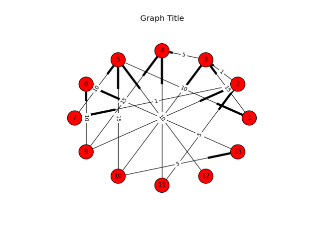
I’ve previously mentioned graphviz for plotting graphs. In truth, these resemble flowcharts. To create something that looks like a more traditional vertex and edge representation, you might consider NetworkX.

Whereas graphviz is a fairly general purpose utility that is not specific to Python and is developed around the well-defined DOT-format, NetworkX is Python specific but creates very nice graphics. It’s also significantly easier to get something that’s acceptable while probably minimizing the amount of time that you have to monkey with it. With that said, there are multiple layout algorithms that you can invoke to calculate the positions of the elements in the output image, and the only apparent way to get a consistent, well-organized/balanced representation seems to arrange them using the circular layout.

Digraph example:

import networkx as nx
import matplotlib.pyplot as plt

def _main():
    g = nx.DiGraph()

    g.add_edge(2, 3, weight=1)
    g.add_edge(3, 4, weight=5)
    g.add_edge(5, 1, weight=10)
    g.add_edge(1, 3, weight=15)

    g.add_edge(2, 7, weight=1)
    g.add_edge(13, 6, weight=5)
    g.add_edge(12, 5, weight=10)
    g.add_edge(11, 4, weight=15)

    g.add_edge(9, 2, weight=1)
    g.add_edge(10, 13, weight=5)
    g.add_edge(7, 5, weight=10)
    g.add_edge(9, 4, weight=15)

    g.add_edge(10, 3, weight=1)
    g.add_edge(11, 2, weight=5)
    g.add_edge(9, 6, weight=10)
    g.add_edge(10, 5, weight=15)

    pos = nx.circular_layout(g)

    edge_labels = { (u,v): d['weight'] for u,v,d in g.edges(data=True) }

    nx.draw_networkx_nodes(g,pos,node_size=700)
    nx.draw_networkx_edges(g,pos)
    nx.draw_networkx_labels(g,pos)
    nx.draw_networkx_edge_labels(g,pos,edge_labels=edge_labels)

    plt.title("Graph Title")
    plt.axis('off')

    plt.savefig('output.png')
    plt.show()

if __name__ == '__main__':
    _main()

Notice that NetworkX depends on matplotlib to do the actual drawing. The boots (highlighted parts on the edges) represent directedness.

Output:

NetworkX

As I said before, it’s easier to get a nicer representation, but it appears that this is at the cost of flexibility. Notice that in the image, there’s a a tendency to overlap. In fact, all of the edge-labels are dead-center. Since the nodes are arranged in a circle, all edges that cross from one side to another will have labels that overlap in the middle. Technically you can adjust whether the label is left, middle, or right, but it’s limited to that (rather than being calculated on the fly).

A Complete Huffman Encoder Implementation

I’ve written a Huffman implementation for the purpose of completely showing how to build the frequency-table, Huffman tree, encoding table, as well as how to serialize the tree, store the tree and data to a file, restore both structures from a file, decode the data using the tree, and how to make this more fun using Python.

This is the test code (test_steps):

clear_bytes = test_get_data()
_dump_hex("Original data:", clear_bytes)

tu = TreeUtility()

# Build encoding table and tree.

he = Encoding()
encoding = he.get_encoding(clear_bytes)

print("Weights:n{0}".format(pprint.pformat(encoding.weights)))
print('')

print("Tree:")
print('')

tu.print_tree(encoding.tree)
print('')

flat_encoding_table = { 
    (hex(c)[2:] + ' ' + chr(c).strip()): b
    for (c, b) 
    in encoding.table.items() }

print("Encoding:n{0}".format(pprint.pformat(flat_encoding_table)))
print('')

# Encode the data.

print("Encoded characters:nn{0}n".
      format(encode_to_debug_string(encoding.table, clear_bytes)))

encoded_bytes = encode(encoding.table, clear_bytes)
_dump_hex("Encoded:", encoded_bytes)

# Decode the data.

decoded_bytes_list = decode(encoding.tree, encoded_bytes)
decoded_bytes = bytes(decoded_bytes_list)

assert 
    clear_bytes == decoded_bytes, 
    "Decoded does not equal the original."

_dump_hex("Decoded:", decoded_bytes)

print("Decoded text:")
print('')
print(decoded_bytes)
print('')

# Serialize and unserialize tree.

serialized_tree = tu.serialize(encoding.tree)
unserialized_tree = tu.unserialize(serialized_tree)

decoded_bytes_list2 = decode(unserialized_tree, encoded_bytes)
decoded_bytes2 = bytes(decoded_bytes_list2)

assert 
    clear_bytes == decoded_bytes2, 
    "Decoded does not equal the original after serializing/" 
    "unserializing the tree."

This is its output:

(Dump) Original data:

54 68 69 73 20 69 73 20 61 20 74 65 73 74 2e 20
54 68 61 6e 6b 20 79 6f 75 20 66 6f 72 20 6c 69
73 74 65 6e 69 6e 67 2e 0a

Weights:
{10: 1,
 32: 7,
 46: 2,
 84: 2,
 97: 2,
 101: 2,
 102: 1,
 103: 1,
 104: 2,
 105: 4,
 107: 1,
 108: 1,
 110: 3,
 111: 2,
 114: 1,
 115: 4,
 116: 3,
 117: 1,
 121: 1}

Tree:

LEFT>
. LEFT>
. . LEFT>
. . . VALUE=(69) [i]
. . RIGHT>
. . . VALUE=(73) [s]
. RIGHT>
. . LEFT>
. . . LEFT>
. . . . VALUE=(54) [T]
. . . RIGHT>
. . . . VALUE=(65) [e]
. . RIGHT>
. . . LEFT>
. . . . LEFT>
. . . . . VALUE=(66) [f]
. . . . RIGHT>
. . . . . VALUE=(72) [r]
. . . RIGHT>
. . . . LEFT>
. . . . . VALUE=(6c) [l]
. . . . RIGHT>
. . . . . VALUE=(a) []
RIGHT>
. LEFT>
. . LEFT>
. . . LEFT>
. . . . VALUE=(6f) [o]
. . . RIGHT>
. . . . VALUE=(61) [a]
. . RIGHT>
. . . LEFT>
. . . . VALUE=(74) [t]
. . . RIGHT>
. . . . VALUE=(6e) [n]
. RIGHT>
. . LEFT>
. . . VALUE=(20) []
. . RIGHT>
. . . LEFT>
. . . . LEFT>
. . . . . LEFT>
. . . . . . VALUE=(6b) [k]
. . . . . RIGHT>
. . . . . . VALUE=(79) [y]
. . . . RIGHT>
. . . . . VALUE=(68) [h]
. . . RIGHT>
. . . . LEFT>
. . . . . VALUE=(2e) [.]
. . . . RIGHT>
. . . . . LEFT>
. . . . . . VALUE=(75) [u]
. . . . . RIGHT>
. . . . . . VALUE=(67) [g]

Encoding:
{'20 ': bitarray('110'),
 '2e .': bitarray('11110'),
 '54 T': bitarray('0100'),
 '61 a': bitarray('1001'),
 '65 e': bitarray('0101'),
 '66 f': bitarray('01100'),
 '67 g': bitarray('111111'),
 '68 h': bitarray('11101'),
 '69 i': bitarray('000'),
 '6b k': bitarray('111000'),
 '6c l': bitarray('01110'),
 '6e n': bitarray('1011'),
 '6f o': bitarray('1000'),
 '72 r': bitarray('01101'),
 '73 s': bitarray('001'),
 '74 t': bitarray('1010'),
 '75 u': bitarray('111110'),
 '79 y': bitarray('111001'),
 'a ': bitarray('01111')}

Encoded characters:

0100 11101 000 001 110 000 001 110 1001 110 1010 0101 001 1010 11110 110 0100 11101 1001 1011 111000 110 111001 1000 111110 110 01100 1000 01101 110 01110 000 001 1010 0101 1011 000 1011 111111 11110 01111

(Dump) Encoded:

4e 83 81 d3 a9 4d 7b 27 66 f8 dc c7 d9 90 dc e0
69 6c 5f fe 7c

(Dump) Decoded:

54 68 69 73 20 69 73 20 61 20 74 65 73 74 2e 20
54 68 61 6e 6b 20 79 6f 75 20 66 6f 72 20 6c 69
73 74 65 6e 69 6e 67 2e 0a

Decoded text:

b'This is a test. Thank you for listening.\n'

Uploading Massive Backups to Amazon Glacier via boto

This is an example of how to use the boto library in Python to perform large, multipart, concurrent uploads to Amazon Glacier.

Notes

  1. The current version of the library (2.38.0) is broken for Python 2.7, for multipart uploads.
  2. The version of the library that we’re using for multipart uploads (2.29.1) is broken for Python 3, as are all other adjacent versions.
  3. Because of (1) and (2), we’re using version 2.29.1 under Python 2.7 and suggest that you do the same.

Example

#!/usr/bin/env python2.7

import os.path

import boto.glacier.layer2

def upload(access_key, secret_key, vault_name, filepath, description):
l = boto.glacier.layer2.Layer2(
aws_access_key_id=access_key,
aws_secret_access_key=secret_key)

v = l.get_vault(vault_name)

archive_id = v.concurrent_create_archive_from_file(
filepath,
description)

print(archive_id)

if __name__ == '__main__':
access_key = 'XXX'
secret_key = 'YYY'
vault_name = 'images'
filepath = '/mnt/array/backups/big_archive.xz'
description = os.path.basename(filepath)

upload(access_key, secret_key, vault_name, filepath, description)

Simple Graphs/DiGraphs with graphviz

We’ll use the graphviz library to generate DOT-formatted data, and the dot command to generate an image:

import subprocess

import graphviz

_RENDER_CMD = ['dot']
_FORMAT = 'png'

def build():
    comment = "Test comment"
    dot = graphviz.Digraph(comment=comment)

    dot.node('P', label='Parent')
    dot.node('G1C1', label='Gen 1 Child 1')
    dot.node('G1C2', label='Gen 1 Child 2')
    dot.node('G2C1', label='Gen 2 Child 1')
    dot.node('G2C2', label='Gen 2 Child 2')

    dot.edge('P', 'G1C1')
    dot.edge('P', 'G1C2')
    dot.edge('G1C2', 'G2C1')
    dot.edge('G1C2', 'G2C2')

    return dot

def get_image_data(dot):
    cmd = _RENDER_CMD + ['-T' + _FORMAT]
    p = subprocess.Popen(
            cmd, 
            stdin=subprocess.PIPE, 
            stdout=subprocess.PIPE, 
            stderr=subprocess.PIPE)

    (stdout, stderr) = p.communicate(input=dot)
    r = p.wait()

    if r != 0:
        raise ValueError("Command failed (%d):n"
                         "Standard output:n%sn"
                         "Standard error:n%s" % 
                         (r, stdout, stderr))

    return stdout

dot = build()
dot_data = get_image_data(dot.source)

with open('output.png', 'wb') as f:
    f.write(dot_data)

GraphViz graph without edge-labels

Note that we can provide labels for the edges, too. However, they tend to crowd the actual edges and it has turned out to be non-trivial to add margins to them:

GraphViz graph with edge-labels

Note that there are other render commands available for different requirements. This list is from the homepage:

  • dot – “hierarchical” or layered drawings of directed graphs. This is the default tool to use if edges have directionality.
  • neato – “spring model” layouts. This is the default tool to use if the graph is not too large (about 100 nodes) and you don’t know anything else about it. Neato attempts to minimize a global energy function, which is equivalent to statistical multi-dimensional scaling.
  • fdp – “spring model” layouts similar to those of neato, but does this by reducing forces rather than working with energy.
  • sfdp – multiscale version of fdp for the layout of large graphs.
  • twopi – radial layouts, after Graham Wills 97. Nodes are placed on concentric circles depending their distance from a given root node.
  • circo – circular layout, after Six and Tollis 99, Kauffman and Wiese 02. This is suitable for certain diagrams of multiple cyclic structures, such as certain telecommunications networks.

This is an example of sfdp with the “-Goverlap=scale” argument with a very large graph (zoomed out).

Example of GraphViz rendered via sfdp

If you’re running OS X, I had to uninstall graphviz, install the gts library, and then reinstall graphviz with an extra option to bind it:

$ brew uninstall graphviz 
$ brew install gts
$ brew install --with-gts graphviz

If graphviz hasn’t been built with gts, you will get the following error:

Standard error:
Error: remove_overlap: Graphviz not built with triangulation library

World’s Simplest Python epoll Example For Waiting on File/Socket Readiness

Once upon a time, the only way to wait to read or write on one or more sockets/descriptors in Linux was the select method, which was later superseded by poll, and then epoll. epoll is the most current and popular way to accomplish this, now. Note that this is only available for Linux, and not for Mac (though select and poll appear to be).

In Python, you can invoke this functionality in the built-in select package. You can use it on any standard system file-descriptor, whether it’s socket-oriented, inotify-related, etc.

import logging
import sys
import socket
import select

_MAX_CONNECTION_BACKLOG = 1
_PORT = 9999
_BINDING = ('0.0.0.0', _PORT)
_EPOLL_BLOCK_DURATION_S = 1

_DEFAULT_LOG_FORMAT = '%(asctime)s - %(name)s - %(levelname)s - %(message)s'

_LOGGER = logging.getLogger(__name__)

_CONNECTIONS = {}

_EVENT_LOOKUP = {
    select.POLLIN: 'POLLIN',
    select.POLLPRI: 'POLLPRI',
    select.POLLOUT: 'POLLOUT',
    select.POLLERR: 'POLLERR',
    select.POLLHUP: 'POLLHUP',
    select.POLLNVAL: 'POLLNVAL',
}

def _configure_logging():
    _LOGGER.setLevel(logging.DEBUG)

    ch = logging.StreamHandler()

    formatter = logging.Formatter(_DEFAULT_LOG_FORMAT)
    ch.setFormatter(formatter)

    _LOGGER.addHandler(ch)

def _get_flag_names(flags):
    names = []
    for bit, name in _EVENT_LOOKUP.items():
        if flags & bit:
            names.append(name)
            flags -= bit

            if flags == 0:
                break

    assert flags == 0, 
           "We couldn't account for all flags: (%d)" % (flags,)

    return names

def _handle_inotify_event(epoll, server, fd, event_type):
    # Common, but we're not interested.
    if (event_type & select.POLLOUT) == 0:
        flag_list = _get_flag_names(event_type)
        _LOGGER.debug("Received (%d): %s", 
                      fd, flag_list)

    # Activity on the master socket means a new connection.
    if fd == server.fileno():
        _LOGGER.debug("Received connection: (%d)", event_type)

        c, address = server.accept()
        c.setblocking(0)

        child_fd = c.fileno()

        # Start watching the new connection.
        epoll.register(child_fd)

        _CONNECTIONS[child_fd] = c
    else:
        c = _CONNECTIONS[fd]

        # Child connection can read.
        if event_type & select.EPOLLIN:
            b = c.recv(1024)
            sys.stdout.write(b)

def _create_server_socket():
    s = socket.socket(socket.AF_INET, socket.SOCK_STREAM)
    s.setsockopt(socket.SOL_SOCKET, socket.SO_REUSEADDR, 1)
    s.bind(_BINDING)
    s.listen(_MAX_CONNECTION_BACKLOG)
    s.setblocking(0)

    return s

def _run_server():
    s = _create_server_socket()

    e = select.epoll()

    # If not provided, event-mask defaults to (POLLIN | POLLPRI | POLLOUT). It 
    # can be modified later with modify().
    e.register(s.fileno())

    try:
        while True:
            events = e.poll(_EPOLL_BLOCK_DURATION_S)
            for fd, event_type in events:
                _handle_inotify_event(e, s, fd, event_type)
    finally:
        e.unregister(s.fileno())
        e.close()
        s.close()

if __name__ == '__main__':
    _configure_logging()
    _run_server()

Now, just connect via telnet to port 9999 on localhost. Submitted text in the client will be printed to the screen on the server:

$ python epoll.py 
2015-04-23 08:34:35,104 - __main__ - DEBUG - Received (3): ['POLLIN']
2015-04-23 08:34:35,104 - __main__ - DEBUG - Received connection: (1)
hello

Writing Custom MySQL Functions

Sometimes, if you spend a lot of time living in the database (using SQL routines and functions), you might either find missing functionality or find that you need to interface to other projects or libraries, directly. You might want to call a stronger random-number generator with a better entropy-source. You might want to invoke a YAML library.

MySQL has a couple of ways to add new functions: native functions (using libraries that are statically-linked into the server) and UDFs (“user-defined functions”, using libraries that are dynamically-linked with the server). Essentially the difference is whether you want to package your functionality into the server or whether you’d be willing to build it, copy it into the right place, and then tell MySQL to import it via a “create” query. In the case of the latter, you’ll have to “drop” it later, first, if it needs to be updated.

We’re going to do a quick run-through of how to write a UDF with MySQL Server 5.5 . For more information on “native” MySQL functions, you can look here. Note that we differentiate between C functions and SQL functions below by referring to the C functions as “native” functions. This is not meant to refer to MySQL’s “native” function support, which will not be referred to after this point.

It’s actually quite simple:

  • Define a native “init” function or a native “deinit” function, or both, to setup and teardown your library.
  • Define the main native function to do the work. You’ll get an array of argument types and values, and use a NULL to determine if you were given a NULL for an argument.
  • Set the (*is_null) parameter to 1 if you’re returning a NULL (but you have to indicate this possibility from the native “init” function).
  • You will return the value directly. If you’re returning a string, set the “length” parameter. You will tell MySQL what type you’re returning when you first import the function.
  • You’ll also have to define native “add” and “clear” functions if you’re writing an aggregate function (e.g. COUNT, SUM, etc..). You’ll be writing an accumulator where values are loaded and then evaluated.

Writing the Plugin

#include <mysql.h>
#include <m_string.h>

#ifdef HAVE_DLOPEN

my_bool testfunc_init(
    UDF_INIT *initid, 
    UDF_ARGS *args, 
    char *message);

longlong testfunc(
    UDF_INIT *initid, 
    UDF_ARGS *args, 
    char *is_null,
    char *error);

my_bool testfunc_init(
    UDF_INIT *initid __attribute__((unused)),
    UDF_ARGS *args __attribute__((unused)),
    char *message __attribute__((unused)))
{
    if(args->arg_count != 1)
    {
        strcpy(message, "testfunc must have exactly one argument.");
        return 1;
    }

    // Allow positive or negative integers.

    if(args->arg_type[0] != REAL_RESULT && 
       args->arg_type[0] != INT_RESULT)
    {
        strcpy(message, "testfunc must have an integer.");
        return 1;
    }

    return 0;
}

longlong testfunc(
    UDF_INIT *initid __attribute__((unused)), 
    UDF_ARGS *args,
    char *is_null __attribute__((unused)),
    char *error __attribute__((unused)))
{
    longlong value;

    if(args->arg_type[0] == REAL_RESULT) 
    {
        value = (longlong)*((double *)args->args[0]);
    }
    else //if(args->arg_type[0] == INT_RESULT)
    {
        value = *((longlong *)args->args[0]);
    }

    return value * 2;
}

#endif

This example SQL function obviously just returns the original integer doubled. The difference between an “integer” and a “real” integer is, also obviously, whether or not the value is negative.

Notes:

  • Plugin support can be disabled in the server. You should check for HAVE_DLOPEN to be defined.
  • Reportedly, at least one of the native “init” or “deinit” functions should be defined.

Building is simple:

$ gcc -shared -o udf_test.so -I /usr/local/Cellar/mysql/5.6.16/include/mysql udf_test.c

Using the Plugin

To use the plugin, copy it into your server’s plugin directory. You can determine this from your server’s variables:

mysql> SHOW VARIABLES LIKE "plugin_dir";
+---------------+--------------------------------------------+
| Variable_name | Value                                      |
+---------------+--------------------------------------------+
| plugin_dir    | /usr/local/Cellar/mysql/5.6.16/lib/plugin/ |
+---------------+--------------------------------------------+
1 row in set (0.00 sec)

To import a function (you may have defined more than one):

mysql> CREATE FUNCTION `testfunc` RETURNS INTEGER SONAME 'udf_test.so';
Query OK, 0 rows affected (0.00 sec)

MySQL will install it into its “func” table:

mysql> SELECT * FROM `mysql`.`func`;
+----------+-----+-------------+----------+
| name     | ret | dl          | type     |
+----------+-----+-------------+----------+
| testfunc |   2 | udf_test.so | function |
+----------+-----+-------------+----------+
1 row in set (0.00 sec)

If you need to unload it (or need to update it and unload it before doing so):

mysql> DROP FUNCTION `testfunc`;
Query OK, 0 rows affected (0.00 sec)

Testing

mysql> SELECT testfunc(111);
+---------------+
| testfunc(111) |
+---------------+
|           222 |
+---------------+
1 row in set (0.00 sec)

For more general information, see 24.3.2 Adding a New User-Defined Function. For more information on arguments, see here. For more information on return values and errors, see 22.3.2.4 UDF Return Values and Error Handling.